A dash of OpenMP goodness

I work on a dual-core dual-socket 1.8 Ghz Opteron at the lab, and was wondering how much performance gain I would get out of a simple OpenMP 'parallel for' invocation...

Turns out that by simply adding this one line, above one of the for loops that controls ray generation, things can get pretty fast:

#pragma omp parallel for num_threads(8)

I have 4 cores, and I did tests with no threading, 4 threads and 8 threads.

Here are the CPU occupancy charts from system monitor:


Single Thread


Four Threads


Eight Threads

Performance:
1 Thread : 78 seconds/frame
4 Threads: 35 seconds/frame
8 Threads: 21 seconds/frame

Of course, the "clock()" function completely messes up in multi-threaded applications, and shows the same time (78 seconds) no matter what the actual time taken is. I measured these off a wall clock.

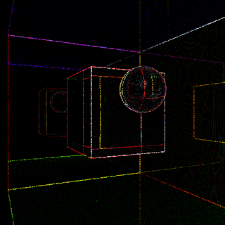
There seems to be some contention, due to which the resultant images for single threaded render and multi-threaded renders are different (by a very very small margin). The diff image has to be enhanced massively to see this. 4 pixels are off by 25%. Many pixels have a difference of 1 color value (out of 255). The images are otherwise undistinguishable to the eye. Need to fix this issue, but I will be taking a break from this project for a while, so updates may come after around 20 days.


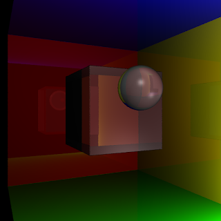
Single Threaded Render


8 Thread Render


25 x Diff image

Ray-bounce improvements and supersampling

2 small updates are in order.

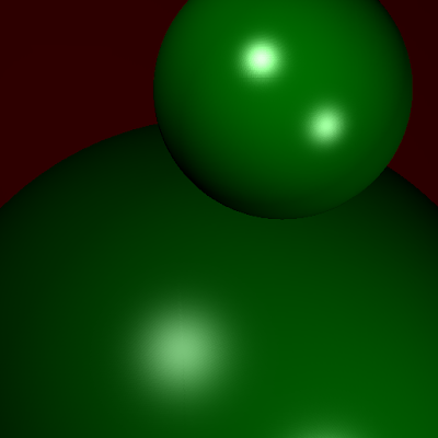
First, the easy one: Anti-aliasing. I have been rendering larger images and downscaling them for achieving antialiasing, but now I added long pending support for multiple random rays per pixel. This way, I can achieve arbitrary sampling rates like 5 rays per pixel, rather than relying on rendering larger and larger images.


No super sampling (3.2 seconds)


8x super sampling (23 seconds)

Of course, nothing nice here, because the running time increases linearly with the number of samples. But here is a theory that I have: on GPUs, larger number of rays per pixel will gather smaller and smaller overhead. Why? Because of ray coherence. Since all these rays travel the same path (mostly), the amount of warp divergence will be very low. In a 2x2 pixel scenario, if we do 8x supersampling for each pixel, the entire warp (8x4 threads) will be well behaved, mostly.

Anyway, now coming to the slightly more obscure improvement. This has to do with an algorithm that I developed for 'seamless' raytracing of point models. Earlier, we had conditions like "if new collision point is within 0.1 units of old collision point of the ray, then ignore this collision point". This is needed because splat based models are not consistent. There can be multiple overlapping splats in the scene, and often, a ray reflected or refracted from one splat, will hit the immediate next splat. This should not happen because its like the ray hitting the same surface twice. Since we are not doing sub-surface scattering :P, we would not like this to happen. But such a naive condition also causes problems with legitimate collisions. For example, we see artifacts at wall corners, and at interfaces of objects where we would expect legitimate ray-hits, but the condition prevents a ray-hit from happening

So, the alternative idea is as follows: Assume the entire scene is made of closed objects. ie: there are no loose hanging objects whose back faces we can see from outside. We add a boolean parameter to each ray, stating which face of an object it would like to hit next (front face or back face). On reflection, this parameter remains same. On refraction, it flips (True to false, false to true). Initially, all primary rays want to hit front faces of objects. Back facing collisions are ignored. Similarly, after the first refraction, objects would like to hit the back face of a splat. This way, we can prevent same-surface collisions. Here is an image illustrating the virtues of this method:


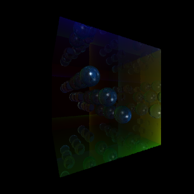
Without Seamless raytracing


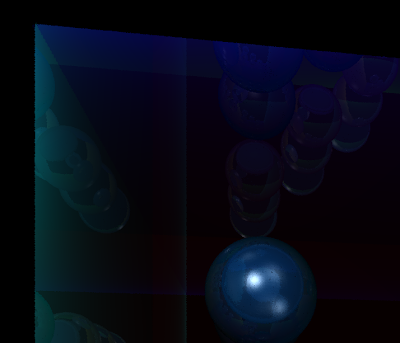
With Seamless raytracing

Eigen2 Debug mode

Eigen's main page claims "Disabling asserts, by defining -DNDEBUG or -DEIGEN_NO_DEBUG, improves performance in some cases."
What they mean is that we need to call g++ with the -DEIGEN_NO_DEBUG option.

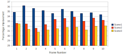
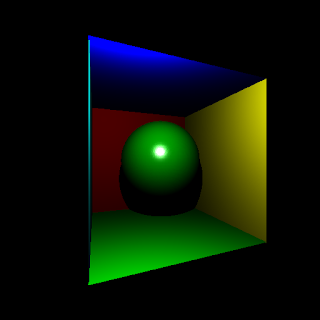
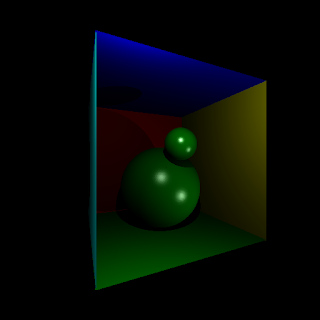
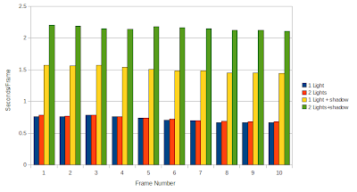
In this post, we test the effect of disabling asserts on a few test scenes. The first scene is a 512x512 render of a refractive sphere with reflective cornell room walls. The second scene is the same room, but 9 refractive spheres. The third scene is obtained by rendering the second scene at 1024x1024 with shadow rays. All scenes have 2 light sources.

Average running times with default settings (eigen in debug mode), were 3.6 seconds for the first scene, 4.3 seconds for the 2nd scene and 47 seconds for the third scene.



This reduces code run times pretty drastically (2.4, 2.8 and 33 seconds approximately for the three scenes described above). There is a clear 30% and above performance improvement when debug mode is disabled. Anyway, debugging with eigen is a nightmare (way too much boilerplate to sift through), and I use my own Vector library while doing serious debugging.

Octree boundary artifacts

I have traced the small artifacts that were popping up in the renders, to issues caused by octree leaf borders. It turns out that an octree border cutting through a smooth surface causes a slice to appear on the surface. This can be seen in the images below. At level 10, there are several small octree nodes, and they cause a large number of slices to appear on the surface. At level 4, there are very few borders of octree nodes, and therefore, we see no artifacts in the render. A more serious side effect is that rays start 'leaking' through the surface at these border points, and cause holes to appear on the surface. In animations, these holes pop in and out in a very distracting manner.


10 level octree (1.2 seconds to render)

8 level octree (1.3 seconds to render)

6 level octree (5 seconds to render)

4 level octree (80 seconds to render)

I don't have a solution to this problem yet, but I am thinking along the lines of adding splats to multiple octree leaves, or checking multiple nearby octree leaves while shading (rather than a single octree leaf).

Shadow Rays

Added a visibility function that works between any 2 points in space (inside or outside the octree).
This means that I can finally implement shadow rays. [Maybe even radiosity :) but that is for another day]

But for the time being, here are the results of shadowing:


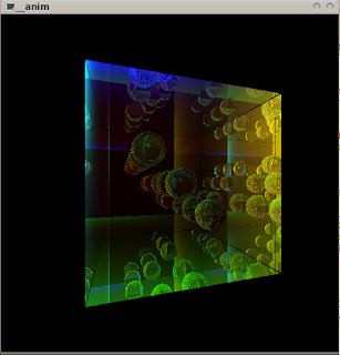
Single Light source


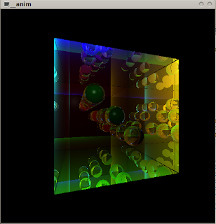
2 Light sources

Shadow rays can be computationally heavy as I found out:


Not much time to spend today, so thats all for now.

Reflection

Reflection, for which functionality was already in place a few days ago, is now working. Here are a few test images. Enabling reflection on all the walls has caused a considerable performance hit. Renders are now around 3 times slower.


Reflective Walls (Max Bounces: 30). Render time: 3.9 seconds

When I say max bounces are 30, it does not mean that all rays bounce 30 times. Most rays don't even make it past 7 or 8 bounces. The reflection coefficient in these images is 0.8 for the walls, and the refraction coefficient for spheres is also 0.8. Rays are traced only while the ray intensity (which starts off as 1.0) is atleast 0.01. Each bounce reduces this 'intensity' value, thereby limiting the number of bounces. So, 30 is just a 'very big number'.


Reflective Walls (Max Bounces: 5). Render Time: 3.16 seconds

Here we see a limited bounce result. With only 5 bounces, the reflections of the spheres lack detail. But we save some time this way.


Diff of 5 and 30 bounce images

Clearly, there is a considerable difference between the two images, but the better image also takes around 20-25% longer to render.


Reduced wall reflection coefficient to 0.4

Here is a more aesthetically pleasing version of the image, with reflection coefficient reduced to 0.4. The diffuse coloring of the walls is more pronounced than the reflections.

Finally, I rendered a high resolution version of the image (4096x4096) and downsampled it (1024x1024) to achieve an anti-aliased image of considerable quality. It took an eternity to render (229 seconds), but looks much better than the 512x512 version.



One small note about the images: You can notice black lines running along the corners of the cornell room. This is because of a 'minimum distance between bounces' threshold that has been set in the code. This prevents rays from bouncing twice off the same surface. Sadly it also has these side effects...

Another issue pending is stochastic reflection and refraction. Currently the system does not support surfaces that both reflect and refract, because rays never spawn off multiple secondary rays. To get this to work, the tracing engine has to trace multiple rays through each pixel. Some of these rays should reflect, and some should refract, depending on the coefficients of reflection and refraction. Monte Carlo integration may help out in blending these results together nicely.

Next on the agenda is splat blending. The refraction results look extremely noisy, and will hopefully benefit from some blending. Also to do is supersampling support, after which we will want adaptive supersampling.

Eigen2 performance

This is a short post on how average runtime of the raytracer is affected when using Eigen2 library (with compiler options O2, msse, msse2), as against rolling your own simple 3D float vector class. I have been using Vector3f from Eigen2, and have not paid any special attention to speed. I just use vectors wherever I can (positions and colors mostly). I have also not bothered about alignment of structures (obviously Vector4f would align properly, but would considerably increase memory requirements).

I was assuming that eigen2 would not give me a significant speed boost, because raytracing is not a compute heavy problem (mostly memory access bound). It turns out that I was wrong:



There is almost a 2x performance gain when I use Eigen2. Very surprising really, because the amount of work it took me is zero. All I had to do was include the right headers. Maybe when I have more time, I will make a branch of the project with Vector4f and see how alignment affects things.

Specularity, Fresnel Terms

Specular Highlight on Opaque Sphere

Here I have used the Blinn-Phong approximation that involves computing the half-vector. The half vector is the sum of the Light and View Vectors, normalized. Dot product of this with the normal, raised to a power (specular coefficient) gives the value of the specular highlight at any point. The higher the power, the more concentrated the spot becomes.


Specular highlight + refraction

You can see that the specular highlight has become slightly dull because the sphere is transparent. Some of the light gets transmitted and some is reflected. This is implemented as a weighted average of the reflected and refracted light, where the weights are the coefficients of transmittance and reflectance.


Constant transmittance on a green sphere

This image shows a sphere with refractive index 1.01, and a transmittance of 0.9 (90% light goes through). The amount of light that gets transmitted is constant all over the sphere.


Fresnel transmittance

This image shows the same sphere, now rendered using Fresnel equations for reflection coefficient. Transmission coefficient is simply 1 - reflection coeffecient. The net effect is that when light is incident perpendicular to a surface, more light gets transmitted than if the ray hits the surface almost parallel to the surface. This can be seen in real life on a water surface. Water from a grazing angle is highly reflective, but when you look at it straight from the top, you can see right through the water. In the above image, this causes the edges of the sphere to be visible, while the rest of the sphere is highly transparent. On increasing the refractive index, the sphere becomes less transparent.

Refractions and more

Added a few basic objects to the raytracer. Now I can create point models of planes, spheres and cylinders with one function call.


Diffuse Sphere

But more importantly, Refraction finally works (I am guessing reflection will work too... but not tested yet). There is considerable aliasing right now.

Here are a few images of the refraction system at work:

9 spheres (1.5 seconds)


Intersecting spheres (2 seconds)


High resolution version (2000x2000, 12.38 seconds)

There are a few issues right now. One is that there seem to be a few rays 'leaking out through walls', due to which you can see black dots. The other is regarding rays that move parallel to the octree leaves. Such rays cannot move forward, because we cannot find their point of intersection with the octree. Adding a check for such rays only slows down the entire process, because such rays are very rare (in the images shown, they turn up as bright white spots). I am still looking for a solution to this issue.

In general, it seems that raytracing is quite hackish too... ie: a lot of messy tweaks are needed to get things working. For example, total internal reflection inside a sphere never terminates. I have a hack which prevents TIR completely, and instead allows the ray to pass through as though nothing ever happened. Then there is the issue of rays hitting overlapping splats which are nearby. Another hack which checks for a minimum distance between collisions, now allows me to avoid the 50 odd collisions that a ray would undergo, while moving through a sphere.

Diffuse Lighting

Cornell Room, with 320000 points (0.6 seconds)

Took some major code refactoring, but I eventually managed to add diffuse lighting to the raytracer.
This includes some major additions like a new Material class, which is now used instead of per splat color values. The Material class has support for ambient, diffuse, specular materials, transparency, etc...

Of course, I also had to add a new light class (PointLight). This is more like a simple struct really.

Then there were a few other changes to incorporate shading. The Material class accepts a light, a position and a normal vector and returns the shaded value. The base class of the entire model, which I call SceneBase, contains a list of pointers to materials and lights. Pointers because then I can easily modify the materials and lights from outside, and things will dynamically change.

SceneBase derives every other scene class. The Octree class has been moved into a container which I call OctreeScene. This gives me an easier way of keeping track of the root node, than to create a global variable called root.

phew... thats a lot of messing around with code to get things working neatly...

Octree Traversal

This post describes a Least common ancestor based Octree traversal algorithm.

Some definitions:

Let us define the concept of 'Wall Owner'. A node is said to "own" a wall, if the wall was created while splitting the node for the first time. Formally,

A node has 6 walls surrounding it. Let us call these as "External Walls" of the node.
When we split a node "n" into 8 parts, we create 3 new walls inside this node. These walls are "Internal Walls". The node "n" is said to be the owner of these walls.

Nobody owns the external nodes of the root. ie: Owner is NULL.

For each child node, three of its walls are owned by the parent (the internal walls).
The remaining 3 walls are External walls of the parent. Who owns these walls? We know this info by asking the parent.

When a ray originates in a leaf node of the octree, we can trace it as follows:

Let the ray hit a wall "W". We know who the owner of this wall is.
We find the intersection point of the ray, on wall W, and slightly advance the ray (by a delta increment), so that the frontier of the ray is now just outside the node.
We now ask the Owner of W, to tell us which leaf node contains this point.
[ This is the improvement that least common ancestors gives us. Otherwise, we would have to traverse each time from the root node ]
Now we just say that the ray originates in this new leaf node, and continue the process.

This is like a 3D line drawing algorithm for an octree. Note that it also works for other non-uniform space partition techniques like KD-trees (there, we have only 2 children per node, hence only one internal wall per node)

It increases the space requirement by 6 pointers per node. We can reduce this to 3 pointers per node + 3 bits (to identify what position each child is in its parent: 0 to 7), because the 3 internal walls need not be stored. The parent is trivially the owner of such walls.

Relation to Naive Octree Tracing:
The algorithm described above can be converted to the naive algorithm, by simply setting the root as the wall owner for all walls. This means, every time we move from one leaf to the neighbouring leaf, we need to traverse the octree from the root node all the way down. If the depth of the octree is large, this can be a significant overhead.

What this new algorithm brings to the table, is the promise of reduced octree traversal overhead. When we move from one node at level 10 to another node at level 10, there is a very low chance of traversing all the way from the root node. We may just go from a level 7 or level 8 parent, back down to level 10. In my experiments with max depth = 10, I have observed 10% to 20% speedup using this algorithm (see the table in previous post).

Memory issue:

The first most obvious drawback is that of extra memory usage. For my test scene (empty Cornell room) consisting of 320,000 points, with a setting of maxdepth=10, and maximum points per leaf = 10, 309,623 nodes were created overall. This means that 0.3 million nodes * 6 walls per node * 4 bytes per wall = 7.2 MB of additional memory was used. The total memory requirement of each octree node is currently 100 bytes (a lot of optimization is in order), of which 24 bytes are due to the walls. Thats almost a factor of 25% increase in memory requirement. We can reduce this to around 13% using the optimization of storing only 3 wall pointers (as described above), in which case the 10-20% speed improvement is at the cost of a 13% memory requirement increase, which may be justified. Of course, using only 3 pointers will add to the number of conditional statements and make the solution a little inelegant, but it just may be worth it. Further tests with larger datasets may swing the argument in favour of this new algorithm.

A fly in the algorithm:
In some situations, the algorithm described above skips a few nodes along the traversal path. How can this occur? Here is a diagram explaining the issue:



This image shows a step in traversal of the octree. We hit the wall of a node (green circle denotes point of intersection), and now want to know which node to traverse next.
To do this, we move a little ahead along the ray so that we get a point that is just outside this wall. We then ask the parent of this node, which node contains the point. In this case, the parent of this node says that the point no longer lies inside it, and so returns null. What we should do in this case is ask the root node where this point is. We could also go step by step upwards, asking the parent of the parent and so on, but I figured we would just waste time that way.

Raytracing at last...

(Red Plane: 10x10 Splats)

(Red Plane: 1600x1600 Splats)

My CPU ray tracer finally works. Um... well, it only traces primary rays right now, and it is single threaded... and there is no filtering... ok ok, its not that big a deal, but I will blog about it anyway :P

The ray tracer is for point based scenes. The only primitive we deal with are splats (points with radii, colour and normal vectors). The acceleration structure is an octree, but I feel the traversal algorithms we use right now can be extended to kd-trees as well. This is my first working ray tracer. It will serve as a precursor to a faster, cooler ray tracer implemented entirely on the GPU. It also provides me with a test bed to debug ideas before implementing them in CUDA.

The octree traversal algorithm is one I came up with last year while doing a quad-tree traversal assignment. It involves storing pointers to nearest common ancestors, at each wall in the tree. Some modifications were required to implement a sparse octree, where empty nodes are not stored at all, but in all, it was not too messy to implement this.

The first thing I noticed about the implementation was that it is still a bit buggy. In the rendering with 1600x1600 points, there seem to be small holes in the plane, where rays are escaping out into the background. It turns out to be a problem caused due to the discretization of space that the octree produces. Some splats have their center in one node, but their radius causes them to 'spill over' into nearby nodes. This is not tracked by the current octree construction algorithm, due to which some splats are missed.

The next thing, which is the cool part is that the code truly seems to run in log(objects) time. The run time for various scene sizes (512x512 render window, no super sampling):

Points	Render Time	Octree Creation Time	Memory	Naive Render Time
10x10	0.39	---	5	0.42
100x100	0.52	0.02	6	0.58
200x200	0.54	0.04	9	0.6
400x400	0.59	0.18	21	0.63
800x800	0.65	0.82	71	0.7
1600x1600	0.7	3.5	271	0.76
5000x5000	0.85	37	1700	??

(Time in seconds, memory in mega bytes)

The timings in the last column refer to the naive algorithm of traversing the tree from the root each time, without using the least common ancestor idea. It turns out to be a very small benefit. Maybe further optimizations are in order...

Of course, there is the memory issue: It takes around 270 MegaBytes for a scene with 2.56 million splats in it. Octree generation also seems to take more time than the actual raytrace, for such large scenes. (We will not go into the details of how much swapping I experienced with the 25 million points scene. I am never running that again)

What remains now is to add the usual raytracing frills like secondary rays, shading, supersampling etc...

"As fast as GLSL"(TM)

Yes, its been a looong time.
So, let me get started with the first item on the menu. I promised to write a "SIMD" version of the diffraction code. It turns out that CUDA gpus do not do 4 wide vector operations (according to a reasonably reliable source). I myself have found no reference to vectorized ALU in the GPU, and all references to SIMD on GPU point to warps, which are in some sense, single instruction multiple data units. So I am now to assume that we can only do scalar operations on each shader unit.

It turns out that we can nevertheless try to squeeze out the requisite performance from CUDA. The GLSL implementation of diffraction through a 256x256 diffraction grating runs in around 5 seconds. It turns out that if we do a single float4 texture read in each iteration of the kernel, and write a float4 at a time to the output buffer, we can save quite some time in the kernel.

The earlier implementations took at best 16.5 seconds to complete the process. The new implementation now just takes 5.6 seconds of which the actual system time is just 4.5 seconds.

Pitfalls:

It turns out that not all is well on the CUDA compiler front. I ran into multiple bugs while implementing this last optimization.
Firstly, I was unable to pass a particular float argument from the cpu code through the kernel, and into 2 device functions. It simply kept mucking up each and every time. I finally gave up and hard-coded that value into the kernel. Later I found that the bug was gone in CUDA 2.3. Not really sure what the bug was, but it may have been related to this next issue.

The CUDA compiler seems to really mess up if you do not EXPLICITLY specify each constant floating point value as single precision (0.65f instead of 0.65). It once in a while throws a warning about 'Double' not being supported. You won't even know where this is because the line number is from the ptx file. Heed this warning and remove all doubles from your code (if you are using g80-g92 that is). These innocuous warnings actually come with drastic side effects.

For example, I had defined a pure function which had a few floating point constants inside it. A single invocation of this function, per iteration in the kernel, would work fine. But 2 or 3 invocations would result in an abrupt return from the kernel, so no processing would be done at all.

Here is the kernel code (brought to you by the magic of vim and :TOhtml)

---

__global__ void gpu_emit_photons(float4* buffer, int inputRow, int inputCol, float pitch)
  {
  const int tid_x = threadIdx.x+blockDim.x*blockIdx.x;//destination col
  const int tid_y = threadIdx.y+blockDim.y*blockIdx.y;//destination row

  float srcPosX, srcPosY, destPosX, destPosY, deltaPosX, deltaPosY;
  const float scrSize_2_inv = 2.0f/screenSize;
  const float lambdaRed = 0.72f, lambdaGreen = 0.53f, lambdaBlue = 0.47f;
  float theta, phi, uRed, vRed, uGreen, vGreen, uBlue, vBlue;
  
  int i,j;
  
  float4 intensity;
  float tempIntensityR = 0.0f, tempIntensityG = 0.0f, tempIntensityB = 0.0f;
  
  for (i=inputRow; i<inputRow+BUCKET_SIZE; i++){
    for (j=inputCol; j<inputCol+BUCKET_SIZE; j++){
      float rand1= -tex2D(texRef1, i, j);
      float rand2= -tex2D(texRef1, i, j+1);

      intensity = tex2D(texRef2, (float)j+rand1, (float)i+rand2);
      srcPosX=posMax*(1.0f- ((float)i+rand1)*scrSize_2_inv);
      srcPosY=posMax*(1.0f- ((float)j+rand2)*scrSize_2_inv);

      destPosX=posMax*(1.0f-(float)tid_x*scrSize_2_inv);
      destPosY=posMax*(1.0f-(float)tid_y*scrSize_2_inv);

    //deltaPos is the difference between x coordinates of src and dest
      deltaPosX=srcPosX-destPosX;
      deltaPosY=srcPosY-destPosY;

      theta = atan2( deltaPosX,screenDistance);
      phi = atan2( deltaPosY,screenDistance);
      
      uRed = theta/lambdaRed; vRed = phi/lambdaRed;
      uGreen = theta/lambdaGreen; vGreen = phi/lambdaGreen;
      uBlue = theta/lambdaBlue; vBlue = phi/lambdaBlue;          

    //Assume light is incident perpendicularly onto the optical element;
    //In the general case, 'u' becomes u-u_input and 'v' becomes v-v_input, where u_input and v_input are angles of incidence
      
      tempIntensityR += wdf_analytical(srcPosX,srcPosY,uRed,vRed,lambdaRed,pitch) * intensity.x;
      tempIntensityG += wdf_analytical(srcPosX,srcPosY,uGreen,vGreen,lambdaGreen,pitch) * intensity.y;
      tempIntensityB += wdf_analytical(srcPosX,srcPosY,uBlue,vBlue,lambdaBlue,pitch) * intensity.z;
      }
    }
    buffer[tid_y + tid_x*SIZE] = buffer[tid_y + tid_x*SIZE] + make_float4(tempIntensityR,tempIntensityG,tempIntensityB,0);
  }

---

In the above code, the function call of interest is wdf_analytical(...). This function evaluates the wigner distribution value at the specified x,y,theta,phi coordinates. Its like a 4d lookup table. We need to invoke this function once for each wavelength of light that we want to handle (here, red, green, blue). It turns out that the simple double to float warning had some unforseen ramifications in terms of crashing my code when the function was called more than once. For a single invocation, it worked like a charm.

Well, now of course, everything is in order, and the code works quite fast. The time for optimizations has almost come to an end. One further optimization I should do before closing the topic however, is to use the Leapfrog Lagged Fibonacci Generator (LLFG random number generator) which a bunch of clever guys at my lab have coded up in CUDA. They claim its the world's fastest random number generator (faster than Mersenne Twister on CUDA). It may give good performance benefits versus using a random texture. Only (a lot of) time will tell...

Optimizing memory access in CUDA

Now that we understand how to use textures in cuda, I think it is time to tackle a simple problem and see how we can optimize some code.

Here is a description of the diffraction problem: There is a NxN input image, and an NxN output image (N is typically 256). Each pixel on the output image receives NxN rays, one from each of the input pixels. Each of these rays deposits the color from the source pixel, modulated by a function (we will call this the transformer function). The transformer is a function of source position (x,y) and direction (theta, phi) of propogation.

The naive implementation is as follows:
1. Put the input image into global memory.
2. Create NxN threads, such that each of these threads operates on one of the output pixels.
3. Each of these threads runs a for loop over all the input pixels. For each ray hitting this output pixel, it computes the intensity and increments the output pixel intensity.

This approach does not scale with image size. For 512x512 image, having such a large for loop inside the kernel is not a good idea... So we will have to think of a more scalable solution:

1. Break the input image into buckets of bxb size, where b is around 8 or 16.
2. Now we have multiple kernel invocations, each one corresponding to a bucket. During each invocation, the threads consider rays only from this small bucket of the input data.

Also, another small complication that we introduce is that to prevent aliasing, we evaluate the intensity at input pixels with small random offsets. To facilitate this, we read in a NxN random buffer. This is also in global memory in the naive implementation.

Naive Implementation, with all global memory reads and writes
Time Taken: 2m11.074s

We try to improve things by using textures for the random array:
Time Taken: 1m47.158s

Then, we use textures even for the input image:
Time Taken: 1m34.969s

Next, we notice that each kernel does bxb computations, thus writing to global memory bxb times. By using a temporary local register to maintain this value, and writing that value only once to global memory, we can save a lot of time:
Time Taken: 0m16.530s

The time shown is for 16x16 buckets. For other bucket sizes:

8x8 : 0m17.117s
32x32: 0m16.592s

Note that the mechanism of using square buckets also ensures locality of reference and therefore makes better use of the texture caches. To really get a sense of the improvement from the original code, a 512x512 evaluation used to take around 20 minutes. and now takes 4m15s.

If you remember from my earlier post about diffraction, I wrote that a 256x256 image is evaluated in around 5 seconds by a GLSL shader implementation. We are now 3x slower than GLSL. The reason for this is that the GLSL code uses vectorization for the RGB components. Using vectorization in CUDA will take good advantage of the SIMD units and hopefully give us the remaining 3x performance boost.

Texture Memory: Any abstraction is bad abstraction

My long battle with CUDA textures has finally come to an end. Who won? Well, it was mostly a compromise. You see, things would go very smoothly if I was not trying to make C++ classes out of everything.

To use textures in CUDA, we first define a channel format descriptor (cudaChannelFormatDesc), and tell it how many bits we want in each texture channel (rgba), and what data format is stored in the textures (signed/unsigned ints, or floats)

cudaChannelFormatDesc channelDesc;
channelDesc = cudaCreateChannelDesc(rBits, gBits, bBits, aBits, datatype);

Then we create the cuda array that stores the data. This is where we decide how big our texture is.

cudaArray* cuArray;
cudaMallocArray(&cuArray, &channelDesc, width, height);

Then we copy the texture data from CPU to GPU:

cudaMemcpyToArray(cuArray, 0, 0, cpuPtr, width*height*sizeof(T), cudaMemcpyHostToDevice);

The final step is to create a texture reference, specify the filtering and addressing modes of this texture (clamped / linear filter / normalized etc...) and bind this reference to the memory that we allocated:

texture<float, 2, cudaReadModeElementType> texRef1;
texRef1.addressMode[0] = cudaAddressModeClamp;
texRef1.addressMode[1] = cudaAddressModeClamp;
texRef1.addressMode[2] = cudaAddressModeClamp;

//Modes: cudaFilterModePoint, cudaFilterModeLinear
texRef1.filterMode = cudaFilterModePoint;

//Normalized addressing means 0 to 1 address, else 0 to width and 0 to height address
texRef1.normalized = false;
cudaBindTextureToArray(texRef1, cuArray, channelDesc);

This texture is read inside the CUDA kernel as follows:

float something = tex2D(texRef1, u, v);

This info can be found anywhere. But now is when things get interesting... The CUDA documentation specifies: "A texture reference is declared at file scope as a variable of type texture".

What this really means is "Thou shalt not make local texture references. Thou shalt also not attempt to pass references around as function parameters. Any attempt to make a texture reference at anything other than translation unit scope shalt be dealt with harshly (by a weird ptx compiler error or by a nvcc crash)." More specifically, you will either see an Open64 compiler crash dump, or a slightly less discouraging PTX error: "State space mismatch between instruction and address in instruction 'tex'"

So, it effectively is Impossible to make a "texReference" class, and put everything into it. The main part, the texture reference itself, should be declared outside the class, at global scope in the same file as your kernel. CRAZY!!

The final abstraction I settled for is this:
template <class T>
class texArrayHandle{
 cudaArray* cuArray;
 cudaChannelFormatDesc channelDesc;
 int width, height;
public: ...
};

The texture reference is still declared outside the class, and the class only hides the creation and destruction of the cudaArray. That is around 50 percent abstraction, and 50 percent C. Atleast, my "create array, save to texture, readback texture" example works. Now, to test this in a 'real world' scenario.

Compiling CUDA projects

I find that a lot of new CUDA developers have this tendency to use the CUDA sdk makefiles (include common.mk), and having loads of dependencies on the cuda utils that the sdk provides. This, in the long run does not seem like a good idea, as it involves depending on what the sdk makefile does, and hence depending on the (heavy) sdk itself. Here is a small tutorial on how to compile stand alone CUDA program with multiple h, cpp and cu files, and a few external headers/libs:

Lets say we have 4 files: main.cpp, test.cpp, test.h, kernel.cu

The idea is that we have to compile the cpp files with g++, and the cu files with nvcc.
Also, we specify that only compilation should take place (no linking), so that if we have any dependencies between files, we won't get zillions of errors.

To do this, compile the cpp files this way:

g++ -c *.cpp

Then compile the cu files:

nvcc -c *.cu

Note that nvcc may not be in your default path. When you install the CUDA toolkit, it is placed in the cuda/bin/nvcc path. For example if you installed cuda toolkit in /usr/local/cuda, then nvcc is in /usr/local/cuda/bin/nvcc. Adding this to your $PATH variable will fix things.

The above steps should produce 3 object files: main.o, test.o, and kernel.o

Finally, link these together and make the final executable:

g++ -o runme *.o

This will link all the object files into a single executable called "runme", which you can run as usual.

To include any specific headers / libraries, simply pass them as arguments during the compile / link phases. For example:

g++ -c -I/usr/local/cuda/include *.cpp
g++ -o runme -L/usr/local/cuda/lib -lcuda -lcudart *.o

While running CUDA programs, you may get a library not found error. To fix this, add the CUDA libraries to your $LD_LIBRARY_PATH environment variable. The libraries are libcuda.so, libcudart.so and will be present in your CUDA toolkit install path.

All this can be condensed into a nice makefile for convenience.

Finally, the part about actually writing CUDA programs that are independent of the SDK. Note that the SDK uses macros like CUT_DEVICE_INIT() which are in practice not needed at all. Simply include the cuda header files, and start making cuda calls.

CUDA Warps and Branching

Hi, Its been a long time since I wrote something here. Over the past week I haven't really been doing much. Read a few papers and tutorials on raytracing / gpu+raytracing... and started on the cpu raytracer framework.

That apart, I have also been experimenting on GPU code and here is a small test I did. It is well documented that current nVidia GPUs have warp sizes of 32 threads and that each thread in a warp should ideally take the same branch. The idea here is that instructions are issued not to each thread, but to each warp. So, if there are 31 threads in a warp that do not have anything to do, and 1 thread that has to do heavy computation, then the entire heavy computation code is issued to all the threads, but these are ignored by the first 31 threads. This causes a delay in execution of the entire warp.

But how bad is this really? Can we verify this as a fact?? Lets find out!

Here is the sample kernel:

__global__ void simulate_gpu()
{
 int idx=blockIdx.x*blockDim.x+threadIdx.x;

 if ( idx % 64 < 32)
  for (int i=idx; i < idx+320; i++){
   double theta1 = sin((double)i / 15);
   double theta2 = sin((double)(i + 1) / 15);
   double theta3 = fmax(theta1, theta2);
   double theta4 = cos( sqrt (10.0 * theta3) );
   double theta5 = pow ( theta3, theta4 );
  }
 else
  for (int i=idx; i < idx+4; i++){
   double theta1 = sin((double)i / 15);
   double theta2 = sin((double)(i + 1) / 15);
   double theta3 = fmax(theta1, theta2);
   double theta4 = cos( sqrt (10.0 * theta3) );
   double theta5 = pow ( theta3, theta4 );
  }
 }


The above if-conditional statement generates a square wave response. the first 32 outcomes are true, next 32 are false, and so on. Note that one of the branches has 320 iterations, while the other branch has only 4 iterations.

The running time for this code for 1994096 kernel executions (including all overheads, as measured using the unix 'time' command), is: 0.872 seconds. (averaged over 4 runs).

Lets modify the condition so it looks like this:


 if ( idx % 32 < 16)


This doubles the frequency of the square wave. So the first 16 outcomes are true, next 16 false, etc...

The running time for this is: 1.370s (again avg over 4 runs). That is around 57% longer than the ideal case.

If this is not convincing enough, lets try something else. Lets remove the branch entirely:


__global__ void simulate_gpu()
{
 int idx=blockIdx.x*blockDim.x+threadIdx.x;

  for (int i=idx; i < idx+320; i++){
   double theta1 = sin((double)i / 15);
   double theta2 = sin((double)(i + 1) / 15);
   double theta3 = fmax(theta1, theta2);
   double theta4 = cos( sqrt (10.0 * theta3) );
   double theta5 = pow ( theta3, theta4 );
  }
 }


This is the part of the earlier branching code that has 320 iterations. Time for execution is 1.394s. That means although half the threads actually execute only 4 iterations, its almost equivalent to evaluating 320 iterations every time, unless your warps are well behaved. The time taken for the remaining half of the branch independently is 0.140s, just to put things into perspective...

Granted, that this way of measuring execution time is not all that accurate... but it goes to show that optimising code to minimise warp divergence is worth it.

Also, what happens if we just miss completely perfect warp control flow? What if one or 2 threads go bad? Lets find out. By setting the frequency of the square wave to slightly less than optimal, (say 62 instead of 64), we can find out how bad it really is. Here are a few such results:


 if ( idx % 62 < 31)


Time reported: 1.063s


 if ( idx % 66 < 33)


Time reported: 1.063s

Hmm, so we don't incur the full penalty. I did a few more tests for smaller numbers (56, 48 etc) and they also report similar execution times...

Next article will hopefully be on memory access optimisations... Once I figure it all out and implement the cuda memory access as C++ convenience classes.

GLSL Diffraction Works!

Finally, the GLSL implementation of the diffraction project is working. Here is a sample image rendered using OpenGL:


The speedup seen is enormous. Lets see how far we have come in terms of efficiency:

Implementation	Number of Rays	Time in seconds
Matlab	2^24	700
CUDA Scatter	2^32	30
CUDA Gather	2^32	10
CUDA Gather+randomize	2^32	30
GLSL gather	2^32	1.5

The reason for such a speedup is mostly because of the number of texture lookups that are performed in the shader. The CUDA application does this using global memory, and that is a lot slower than texture lookups (because textures use the texture caches present in hardware).

An interesting issue that pops up here is that each shader kernel should complete in a very short duration of time (around 5 to 10 seconds). I have not found any reference to this online, but I have seen this messing with the results for 2^36 rays. It seems to be similar to the CUDA limit of around 5 to 10 seconds per kernel execution. One solution is to come up with shorter kernels, and another option is to run the application on a GPU that is not connected to an X-server. Since running GLSL on such a (offline) GPU is out of question, I guess I am back to smaller kernels, or implementing the whole thing in CUDA using texture memory.

Note: For people who want to try out large kernels in GLSL/CUDA, a warning: running such kernels will make your system unresponsive for the entire duration, and may as well cause display corruption. I have lost count of the system restarts I have had to do in such cases... You will know that your kernel is taking too much time, if you get garbled results like this one here:

Today's agenda

1. Read up on textures in CUDA, and implement to see how much faster the diffraction kernel becomes.

2. Try to get the shader version working. Some bugs in the code right now cause the output to be a black screen. The processing is happening though... because the computer hangs for around 5 seconds while the shader executes...

For this, I will be using the "Adaptive tessellation for displacement mapping" source that I wrote with Rohit as the code base.

3. Purcell's PhD thesis is still elusive :)

Updated Diffraction results

My attempts at random sampling have been *partially* successful.

Here is the original Mona Lisa Image:


This is the image after diffraction through a cloth of 100 micron weave. This image is generated through uniform sampling (as shown in the preliminary paper submitted to Siggraph asia):


This is the result of using random sampling to randomize ray source positions. The same random numbers are used for each row of the image, which gives it a striped look:


Finally, using better quality random numbers (random throughout the image, not just across a row):


Performance tradeoffs:

The random sampling in CUDA has been implemented as a lookup into a 1D array of random numbers passed by the CPU to the GPU. This means two additional lookups from a global memory array. It drastically reduces the execution speed from around 33 seconds (no randomization) to 90 seconds (with 2 random number lookups). This heavy performance hit can be attributed (IMO) to slow global memory read. Hopefully with 1D texture lookups, this will be mitigated.

The next step is to add bilinear texture sampling at these random source points. Currently, I use no filtering for the texture lookup. This means learning how to use textures in CUDA. Another avenue I am exploring is writing a GLSL shader to do the same. Preliminary results are very promising (around 5 seconds for the entire process, as compared to 33 seconds on CUDA).

cudaThreadSynchronize

This function is important for anyone who is launching a kernel many times (example: from a for loop). This is because a CUDA kernel launch is asynchronous, and returns immediately. This means that your CPU side for loop will finish in an instant and try to launch everything at once.

Calling cudaThreadSynchronize() will make the CPU wait till all previously launched kernels terminate.

Day 1

Wishlist:

1. Fix the CUDA code for Augmented photon mapping (Diffraction code).
Currently the code performs uniform, regular sampling of the diffracting surface. Adding some randomness should improve things on the aliasing front.

2. Port the code to C++ (the last test on cpu was on matlab, which doesnt really count towards efficient processing). Learn how to use OpenMP and go all out on the dual socket opteron.

3. Read Tim Purcell's Raytracing on Stream Processors PhD thesis. This is a slightly longer term plan (ie: over 3 to 4 days)

Rays of hope

Congratulations! You have just found my short-term To-Do list!

(Oh, you were looking for a blog? Sorry, but this is the bitter truth. No blog here.)

My productivity over the last few weeks has been appalling at best. So, before I spend the rest of my life clueless as to what is happening to me, I will start blogging about my day... well, at least the work part of it ;)

...which brings me to my work. For the next year or so, I will be (trying) to develop a realtime raytracer for point models. And to make things spicier, lets throw a few GPUs (Graphics cards) into the soup.

So, in short, you will see my tiny experiments on anything vaguely relevant to raytracing, parallel processing, GPU programming, and computer graphics in general.